1
2
3
4
5
6
7
8
9
10
11
12
13
14
15
16
17
18
19
20
21
22
23
24
25
26
27
28
29
30
31
32
33
34
35
36
37
38
39
40
41
42
43
44
45
46
47
48
49
50
51
52
|
clear all; close all;
N=50;
M=100;
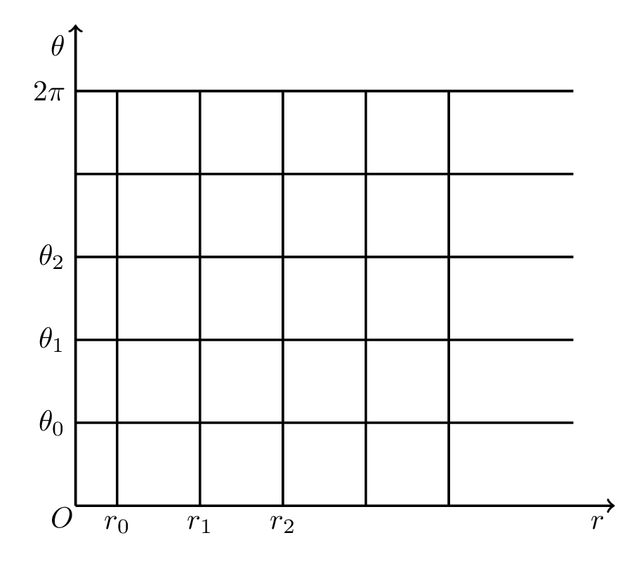
dr=1/(N+1/2);
dthe=2*pi/M;
r=(dr/2:dr:1)';
the=(0:dthe:2*pi)';
[The,R]=meshgrid(the,r);
The1=The(1:N,2:end); R1=R(1:N,2:end);
f=2*R1.*(sin(The1)+cos(The1));
f=f';
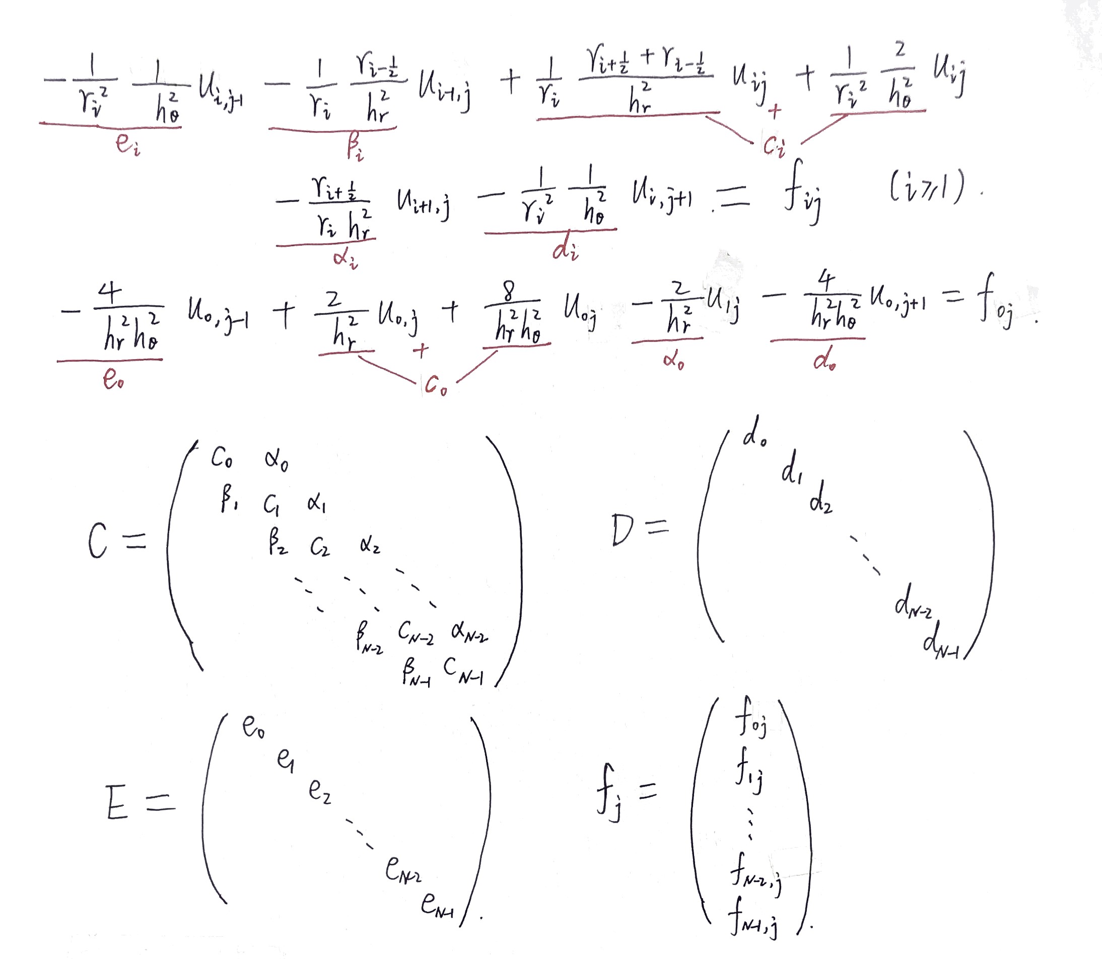
e=[2/dr^2+8/(dr^2*dthe^2);(2./(dthe^2*r(2:N).^2)+2/dr^2)];
e1=[-2/dr^2;-(r(2:N-1)+dr/2)./(dr^2*r(2:N-1))];
e2=-(r(2:N)-dr/2)./(dr^2*r(2:N));
C=diag(e)+diag(e1,1)+diag(e2,-1);
D=diag([-4/(dr^2*dthe^2);-1./(dthe^2*r(2:N).^2)]);
E=diag([-4/(dr^2*dthe^2);-1./(dthe^2*r(2:N).^2)]);
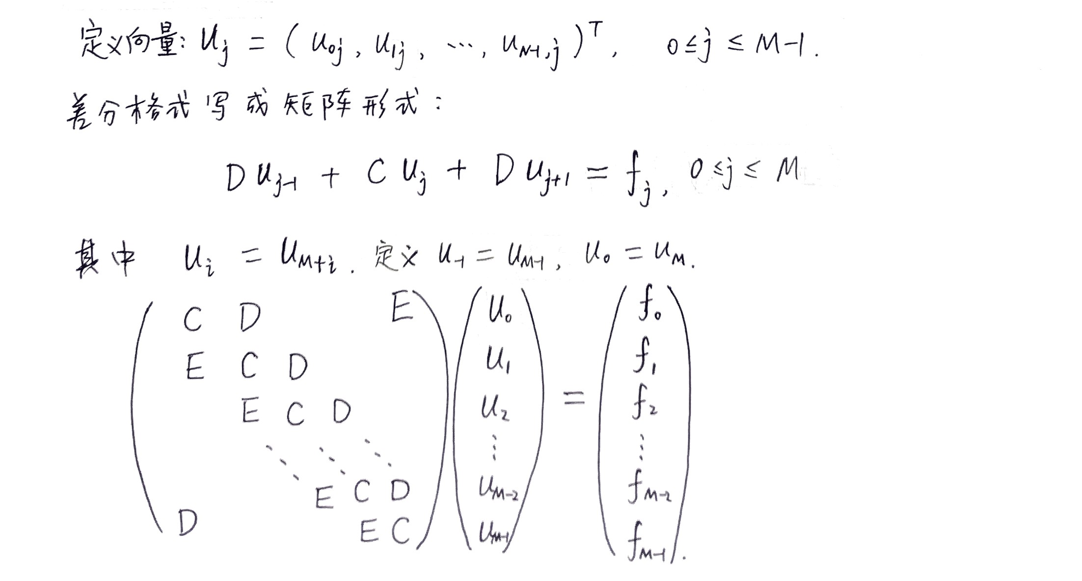
A=kron(eye(M),C)+kron(diag(ones(M-1,1),1)+diag(1,1-M),D)...
+kron(diag(ones(M-1,1),-1)+diag(1,M-1),E);
f=f';
uh=reshape(A\f(:),N,M);
un=[uh;zeros(1,M)];
un=[un(:,end),un];
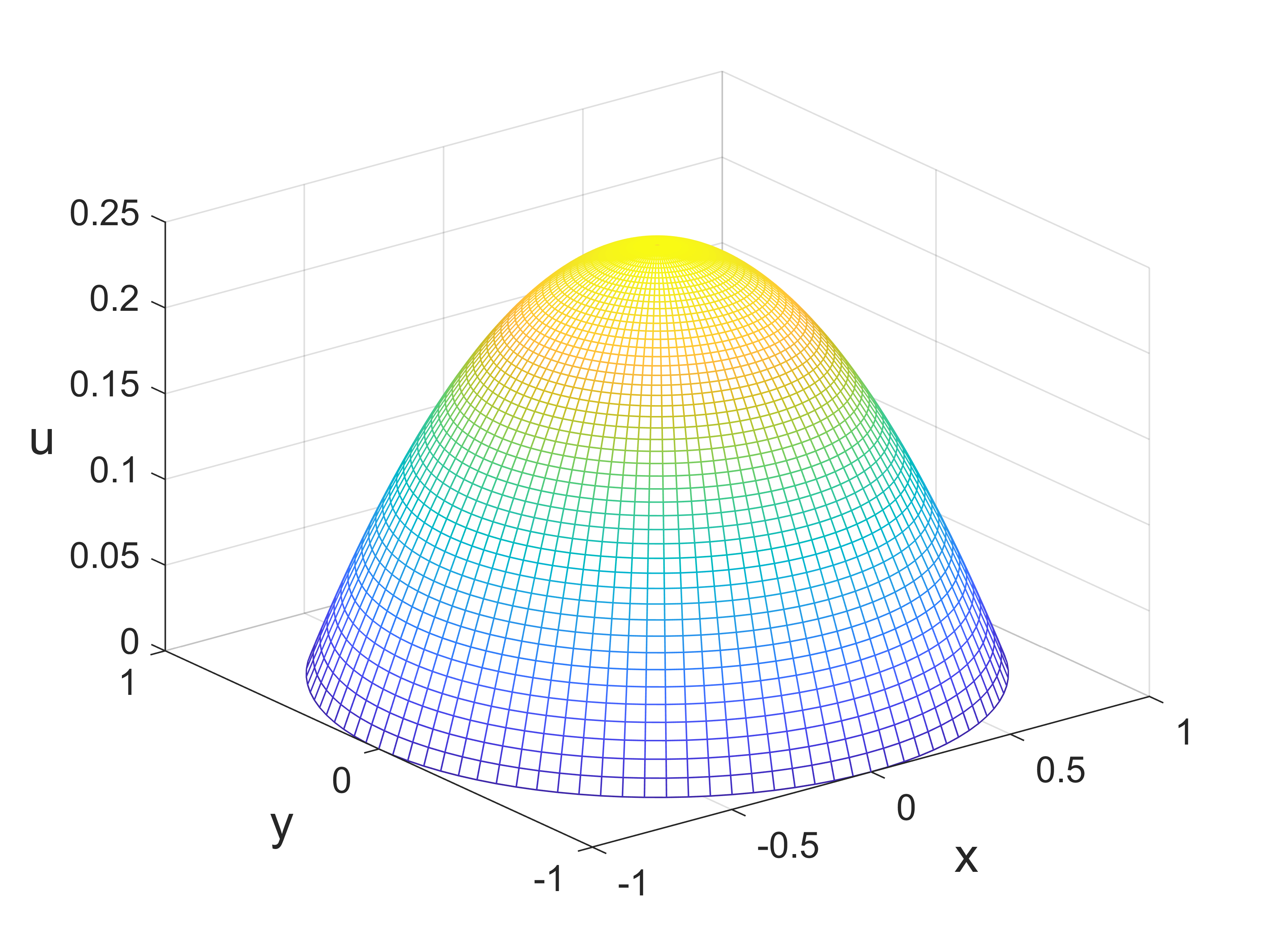
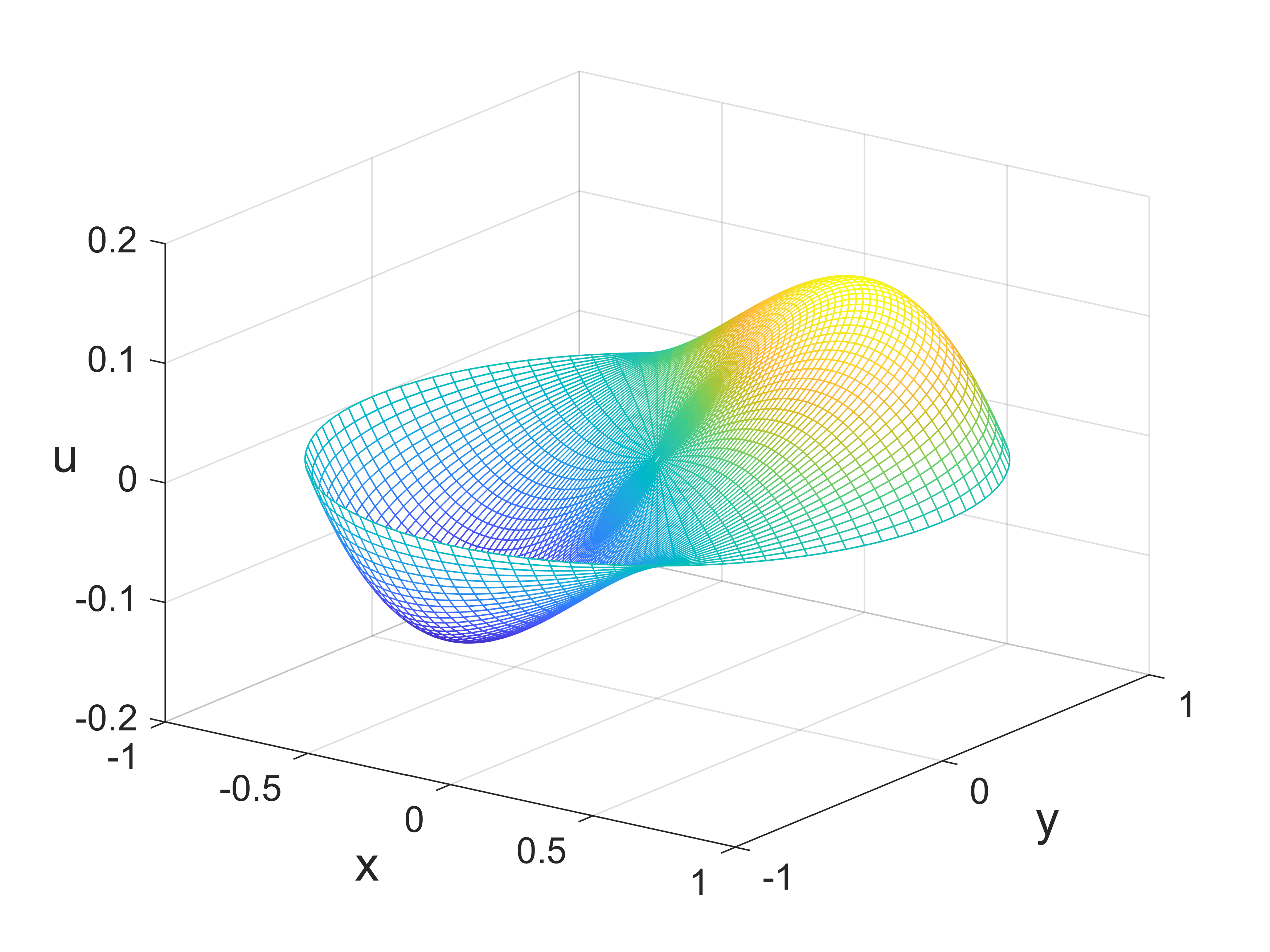
ue=(1-R.^2).*R.*(sin(The)+cos(The))/4;
Err=abs(un(1:N,2:end)-ue(1:N,2:end));
MaxErr=max(max(abs(un-ue)))
[X,Y] = pol2cart(The,R);
mesh(X,Y,ue)
set(gca,'fontsize',12)
xlabel('x','fontsize', 16)
ylabel('y','fontsize',16)
zlabel('u','fontsize',16)
view(36,24)
|